Moderation (statistics) on:
[Wikipedia]
[Google]
[Amazon]
In

 Moderation analysis in the
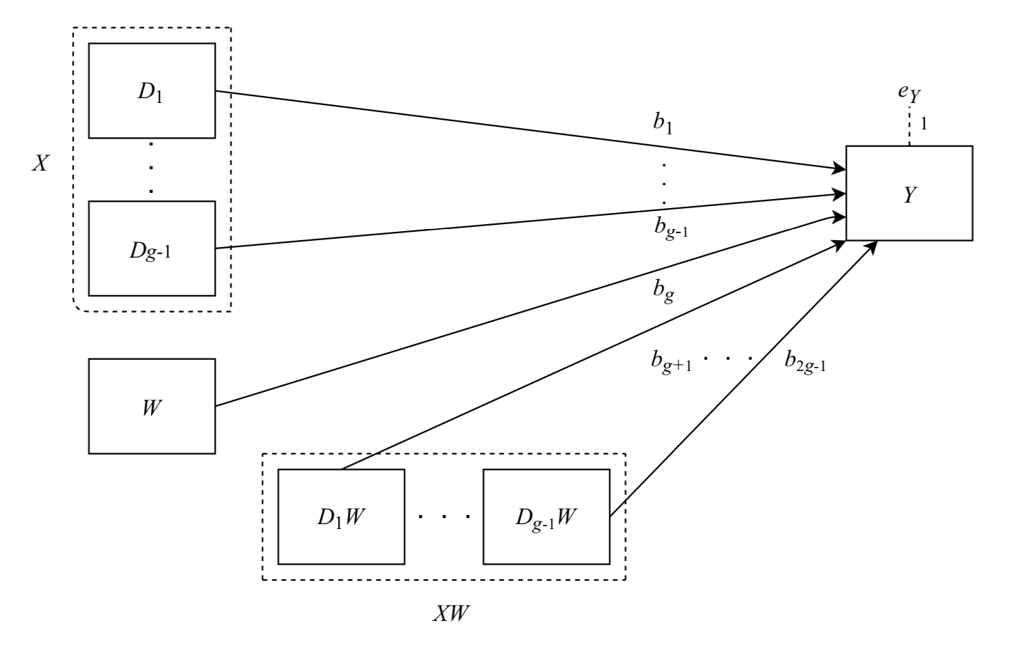 If the first independent variable is a categorical variable (e.g. gender) and the second is a continuous variable (e.g. scores on the Satisfaction With Life Scale (SWLS)), then b1 represents the difference in the dependent variable between males and females when
  Cohen et al. (2003) recommended using the following to probe the simple effect of gender on the dependent variable (Y) at three levels of the continuous independent variable: high (one standard deviation above the mean), moderate (at the mean), and low (one standard deviation below the mean). If the scores of the continuous variable are not standardized, one can just calculate these three values by adding or subtracting one standard deviation of the original scores; if the scores of the continuous variable are standardized, one can calculate the three values as follows: high = the standardized score minus 1, moderate (mean = 0), low = the standardized score plus 1. Then one can explore the effects of gender on the dependent variable (''Y'') at high, moderate, and low levels of the SWLS score. As with two categorical independent variables, ''b''2 represents the effect of the SWLS score on the dependent variable for females. By reverse coding the gender variable, one can get the effect of the SWLS score on the dependent variable for males.

 When treating categorical variables such as ethnic groups and experimental treatments as independent variables in moderated regression, one needs to code the variables so that each code variable represents a specific setting of the categorical variable. There are three basic ways of coding: Dummy-variable coding, Effects coding, and Contrast coding. Below is an introduction to these coding systems.
 Dummy coding is used when one has a reference group or one condition in particular (e.g. a control group in the experiment) that is to be compared to each of the other experimental groups. In this case, the intercept is the mean of the reference group, and each of the unstandardized regression coefficients is the difference in the dependent variable between one of the treatment groups and the mean of the reference group (or control group). This coding system is similar to ANOVA analysis, and is appropriate when researchers have a specific reference group and want to compare each of the other groups with it.
Effects coding is used when one does not have a particular comparison or control group and does not have any planned orthogonal contrasts. The intercept is the grand mean (the mean of all the conditions). The regression coefficient is the difference between the mean of one group and the mean of all the group means (e.g. the mean of group A minus the mean of all groups). This coding system is appropriate when the groups represent natural categories.
Contrast coding is used when one has a series of orthogonal contrasts or group comparisons that are to be investigated. In this case, the intercept is the unweighted mean of the individual group means. The unstandardized regression coefficient represents the difference between the unweighted mean of the means of one group (A) and the unweighted mean of another group (B), where A and B are two sets of groups in the contrast. This coding system is appropriate when researchers have an a priori hypothesis concerning the specific differences among the group means.
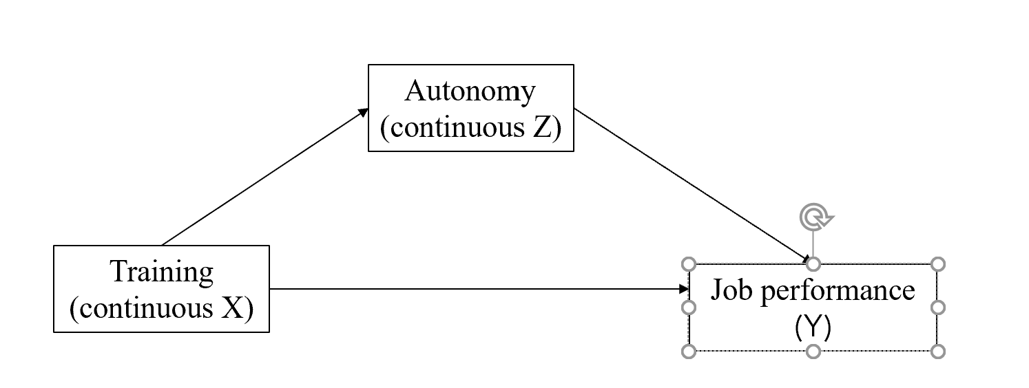
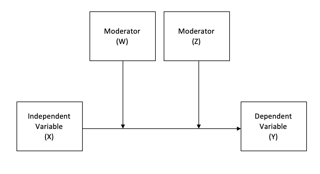
 If both of the independent variables are continuous, it is helpful for interpretation to either center or standardize the independent variables, ''X'' and ''Z''. (Centering involves subtracting the overall sample mean score from the original score; standardizing does the same followed by dividing by the overall sample standard deviation.) By centering or standardizing the independent variables, the coefficient of ''X'' or ''Z'' can be interpreted as the effect of that variable on Y at the mean level of the other independent variable.
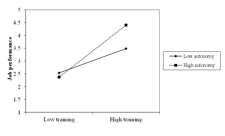
To probe the interaction effect, it is often helpful to plot the effect of ''X'' on ''Y'' at low and high values of ''Z'' (some people prefer to also plot the effect at moderate values of ''Z'', but this is not necessary). Often values of ''Z'' that are one standard deviation above and below the mean are chosen for this, but any sensible values can be used (and in some cases there are more meaningful values to choose). The plot is usually drawn by evaluating the values of ''Y'' for high and low values of both ''X'' and ''Z'', and creating two lines to represent the effect of ''X'' on ''Y'' at the two values of ''Z''. Sometimes this is supplemented by simple slope analysis, which determines whether the effect of ''X'' on ''Y'' is
statistics
Statistics (from German language, German: ''wikt:Statistik#German, Statistik'', "description of a State (polity), state, a country") is the discipline that concerns the collection, organization, analysis, interpretation, and presentation of ...
and regression analysis
In statistical modeling, regression analysis is a set of statistical processes for estimating the relationships between a dependent variable (often called the 'outcome' or 'response' variable, or a 'label' in machine learning parlance) and one ...
, moderation (also known as effect modification) occurs when the relationship between two variables depends on a third variable. The third variable is referred to as the moderator variable (or effect modifier) or simply the moderator (or modifier). The effect of a moderating variable is characterized statistically as an interaction; that is, a categorical (e.g., sex, ethnicity, class) or continuous
Continuity or continuous may refer to:
Mathematics
* Continuity (mathematics), the opposing concept to discreteness; common examples include
** Continuous probability distribution or random variable in probability and statistics
** Continuous ...
(e.g., age, level of reward) variable
Variable may refer to:
* Variable (computer science), a symbolic name associated with a value and whose associated value may be changed
* Variable (mathematics), a symbol that represents a quantity in a mathematical expression, as used in many ...
that is associated with the direction and/or magnitude of the relation between dependent and independent variables
Dependent and independent variables are variables in mathematical modeling, statistical modeling and experimental sciences. Dependent variables receive this name because, in an experiment, their values are studied under the supposition or demand ...
. Specifically within a correlation
In statistics, correlation or dependence is any statistical relationship, whether causal or not, between two random variables or bivariate data. Although in the broadest sense, "correlation" may indicate any type of association, in statistics ...
al analysis framework, a moderator is a third variable that affects the zero-order correlation between two other variables, or the value of the slope of the dependent variable on the independent variable. In analysis of variance
Analysis of variance (ANOVA) is a collection of statistical models and their associated estimation procedures (such as the "variation" among and between groups) used to analyze the differences among means. ANOVA was developed by the statisticia ...
(ANOVA) terms, a basic moderator effect can be represented as an interaction
Interaction is action that occurs between two or more objects, with broad use in philosophy and the sciences. It may refer to:
Science
* Interaction hypothesis, a theory of second language acquisition
* Interaction (statistics)
* Interactions o ...
between a focal independent
Independent or Independents may refer to:
Arts, entertainment, and media Artist groups
* Independents (artist group), a group of modernist painters based in the New Hope, Pennsylvania, area of the United States during the early 1930s
* Independ ...
variable and a factor that specifies the appropriate conditions for its operation.
Example

 Moderation analysis in the
 behavioral sciences
Behavioral sciences explore the cognitive processes within organisms and the behavioral interactions between organisms in the natural world. It involves the systematic analysis and investigation of human and animal behavior through naturalistic o ...
involves the use of linear multiple regression analysis or causal modelling. To quantify the effect of a moderating variable in multiple regression analyses, regressing random variable
A random variable (also called random quantity, aleatory variable, or stochastic variable) is a mathematical formalization of a quantity or object which depends on random events. It is a mapping or a function from possible outcomes (e.g., the po ...
''Y'' on ''X'', an additional term is added to the model. This term is the interaction between ''X'' and the proposed moderating variable.
Thus, for a response ''Y'' and two variables ''x''1 and moderating variable ''x''2,:
:
In this case, the role of ''x''2 as a moderating variable is accomplished by evaluating ''b''3, the parameter estimate for the interaction term. See linear regression
In statistics, linear regression is a linear approach for modelling the relationship between a scalar response and one or more explanatory variables (also known as dependent and independent variables). The case of one explanatory variable is call ...
for discussion of statistical evaluation of parameter estimates in regression analyses.
Multicollinearity in moderated regression
In moderated regression analysis, a newinteraction
Interaction is action that occurs between two or more objects, with broad use in philosophy and the sciences. It may refer to:
Science
* Interaction hypothesis, a theory of second language acquisition
* Interaction (statistics)
* Interactions o ...
predictor () is calculated. However, the new interaction term will be correlated with the two main effects terms used to calculate it. This is the problem of multicollinearity
In statistics, multicollinearity (also collinearity) is a phenomenon in which one predictor variable in a multiple regression model can be linearly predicted from the others with a substantial degree of accuracy. In this situation, the coeffic ...
in moderated regression. Multicollinearity tends to cause coefficients to be estimated with higher standard error
The standard error (SE) of a statistic (usually an estimate of a parameter) is the standard deviation of its sampling distribution or an estimate of that standard deviation. If the statistic is the sample mean, it is called the standard error ...
s and hence greater uncertainty.
Mean-centering (subtracting raw scores from the mean) can reduce multicollinearity, resulting in more interpretable regression coefficients. However, it does not affect the overall model fit.
Post-hoc probing of interactions
Like simple main effect analysis in ANOVA, in post-hoc probing of interactions in regression, we are examining the simple slope of one independent variable at the specific values of the other independent variable. Below is an example of probing two-way interactions. In what follows the regression equation with two variables A and B and an interaction term A*B, : will be considered.Two categorical independent variables
If both of the independent variables are categorical variables, we can analyze the results of the regression for one independent variable at a specific level of the other independent variable. For example, suppose that both A and B are single dummy coded (0,1) variables, and that A represents ethnicity (0 = European Americans, 1 = East Asians) and B represents the condition in the study (0 = control, 1 = experimental). Then the interaction effect shows whether the effect of condition on the dependent variable Y is different for European Americans and East Asians and whether the effect of ethnic status is different for the two conditions. The coefficient of A shows the ethnicity effect on Y for the control condition, while the coefficient of B shows the effect of imposing the experimental condition for European American participants. To probe if there is any significant difference between European Americans and East Asians in the experimental condition, we can simply run the analysis with the condition variable reverse-coded (0 = experimental, 1 = control), so that the coefficient for ethnicity represents the ethnicity effect on Y in the experimental condition. In a similar vein, if we want to see whether the treatment has an effect for East Asian participants, we can reverse code the ethnicity variable (0 = East Asians, 1 = European Americans).One categorical and one continuous independent variable
 If the first independent variable is a categorical variable (e.g. gender) and the second is a continuous variable (e.g. scores on the Satisfaction With Life Scale (SWLS)), then b1 represents the difference in the dependent variable between males and females when
 life satisfaction
Life satisfaction is a measure of a person's well-being, assessed in terms of mood, relationship satisfaction, achieved goals, self-concepts, and self-perceived ability to cope with life. Life satisfaction involves a favorable attitude towards on ...
is zero. However, a zero score on the Satisfaction With Life Scale is meaningless as the range of the score is from 7 to 35. This is where centering comes in. If we subtract the mean of the SWLS score for the sample from each participant's score, the mean of the resulting centered SWLS score is zero. When the analysis is run again, b1 now represents the difference between males and females at the mean level of the SWLS score of the sample.
 Cohen et al. (2003) recommended using the following to probe the simple effect of gender on the dependent variable (Y) at three levels of the continuous independent variable: high (one standard deviation above the mean), moderate (at the mean), and low (one standard deviation below the mean). If the scores of the continuous variable are not standardized, one can just calculate these three values by adding or subtracting one standard deviation of the original scores; if the scores of the continuous variable are standardized, one can calculate the three values as follows: high = the standardized score minus 1, moderate (mean = 0), low = the standardized score plus 1. Then one can explore the effects of gender on the dependent variable (''Y'') at high, moderate, and low levels of the SWLS score. As with two categorical independent variables, ''b''2 represents the effect of the SWLS score on the dependent variable for females. By reverse coding the gender variable, one can get the effect of the SWLS score on the dependent variable for males.
Coding in moderated regression

 When treating categorical variables such as ethnic groups and experimental treatments as independent variables in moderated regression, one needs to code the variables so that each code variable represents a specific setting of the categorical variable. There are three basic ways of coding: Dummy-variable coding, Effects coding, and Contrast coding. Below is an introduction to these coding systems.
 Dummy coding is used when one has a reference group or one condition in particular (e.g. a control group in the experiment) that is to be compared to each of the other experimental groups. In this case, the intercept is the mean of the reference group, and each of the unstandardized regression coefficients is the difference in the dependent variable between one of the treatment groups and the mean of the reference group (or control group). This coding system is similar to ANOVA analysis, and is appropriate when researchers have a specific reference group and want to compare each of the other groups with it.
Effects coding is used when one does not have a particular comparison or control group and does not have any planned orthogonal contrasts. The intercept is the grand mean (the mean of all the conditions). The regression coefficient is the difference between the mean of one group and the mean of all the group means (e.g. the mean of group A minus the mean of all groups). This coding system is appropriate when the groups represent natural categories.
Contrast coding is used when one has a series of orthogonal contrasts or group comparisons that are to be investigated. In this case, the intercept is the unweighted mean of the individual group means. The unstandardized regression coefficient represents the difference between the unweighted mean of the means of one group (A) and the unweighted mean of another group (B), where A and B are two sets of groups in the contrast. This coding system is appropriate when researchers have an a priori hypothesis concerning the specific differences among the group means.
Two continuous independent variables


 If both of the independent variables are continuous, it is helpful for interpretation to either center or standardize the independent variables, ''X'' and ''Z''. (Centering involves subtracting the overall sample mean score from the original score; standardizing does the same followed by dividing by the overall sample standard deviation.) By centering or standardizing the independent variables, the coefficient of ''X'' or ''Z'' can be interpreted as the effect of that variable on Y at the mean level of the other independent variable.
To probe the interaction effect, it is often helpful to plot the effect of ''X'' on ''Y'' at low and high values of ''Z'' (some people prefer to also plot the effect at moderate values of ''Z'', but this is not necessary). Often values of ''Z'' that are one standard deviation above and below the mean are chosen for this, but any sensible values can be used (and in some cases there are more meaningful values to choose). The plot is usually drawn by evaluating the values of ''Y'' for high and low values of both ''X'' and ''Z'', and creating two lines to represent the effect of ''X'' on ''Y'' at the two values of ''Z''. Sometimes this is supplemented by simple slope analysis, which determines whether the effect of ''X'' on ''Y'' is
 statistically significant
In statistical hypothesis testing, a result has statistical significance when it is very unlikely to have occurred given the null hypothesis (simply by chance alone). More precisely, a study's defined significance level, denoted by \alpha, is the p ...
at particular values of ''Z''. Various internet-based tools exist to help researchers plot and interpret such two-way interactions.

Higher-level interactions
The principles for two-way interactions apply when we want to explore three-way or higher-level interactions. For instance, if we have a three-way interaction between ''A'', ''B'', and ''C'', the regression equation will be as follows: :Spurious higher-order effects
It is worth noting that the reliability of the higher-order terms depends on the reliability of the lower-order terms. For example, if the reliability for variable A is 0.70, and reliability for variable B is 0.80, then the reliability for the interaction variable A * B is 0.70 × 0.80 = 0.56. In this case, low reliability of the interaction term leads to low power; therefore, we may not be able to find the interaction effects between A and B that actually exist. The solution for this problem is to use highly reliable measures for each independent variable. Another caveat for interpreting the interaction effects is that when variable A and variable B are highly correlated, then the A * B term will be highly correlated with the omitted variable A2; consequently what appears to be a significant moderation effect might actually be a significant nonlinear effect of A alone. If this is the case, it is worth testing a nonlinear regression model by adding nonlinear terms in individual variables into the moderated regression analysis to see if the interactions remain significant. If the interaction effect A*B is still significant, we will be more confident in saying that there is indeed a moderation effect; however, if the interaction effect is no longer significant after adding the nonlinear term, we will be less certain about the existence of a moderation effect and the nonlinear model will be preferred because it is more parsimonious. Moderated regression analyses also tend to include additional variables, which are conceptualized as covariates of no interest. However, the presence of these covariates can induce spurious effects when either (1) the covariate (C) is correlated with one of the primary variables of interest (e.g. variable A or B), or (2) when the covariate itself is a moderator of the correlation between either A or B with Y. The solution is to include additional interaction terms in the model, for the interaction between each confounder and the primary variables as follows:See also
*Omitted-variable bias
In statistics, omitted-variable bias (OVB) occurs when a statistical model leaves out one or more relevant variables. The bias results in the model attributing the effect of the missing variables to those that were included.
More specifically, OV ...
References
* Hayes, A. F., & Matthes, J. (2009). "Computational procedures for probing interactions in OLS and logistic regression: SPSS and SAS implementations." Behavior Research Methods, Vol. 41, pp. 924–936. {{Statistics Regression analysis